AE

自编码器包含一个编码器和解码器，训练得到的中间特征表示 $z$ 概括了数据的绝大部分信息，是一种良好的特征表示，可以应用于下游任务或者达到数据降维的目的。但AE模型有个显著的缺点是难以从隐变量中采样生成新的数据，网络并没有显式地学习 $z$ 的分布。后续发展的变分自编码器弥补了这一短板。

VAE

VAE中约束了编码向量 $z$ ，训练过程中使 $z$ 服从标准正太分布来达成采样生成的目的。

VAE的核心是变分推断，最初是用于估计难以积分计算的后验概率 $p(z|x)$ ——使用分布族里的分布逼近后验分布，将后验概率的求解问题转化为了一个优化问题。

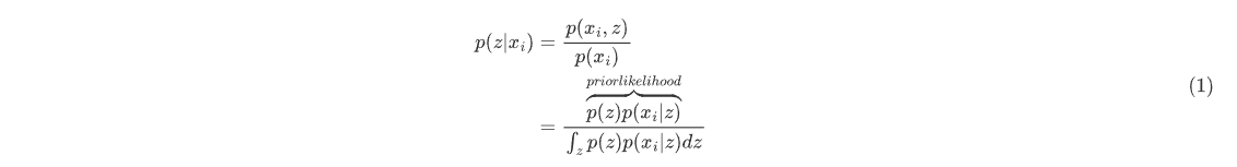
其中 $p(z)$ 和 $ p(x|z) $ 分别为先验和似然分布，分母处的高维积分是难以求解的，这就导致我们难以找出后验分布的解析解形式。

变分法：利用 $q(z)$ 逼近 $p(z|x)$ ，这里选择高斯分布族进行逼近便于计算和推导。

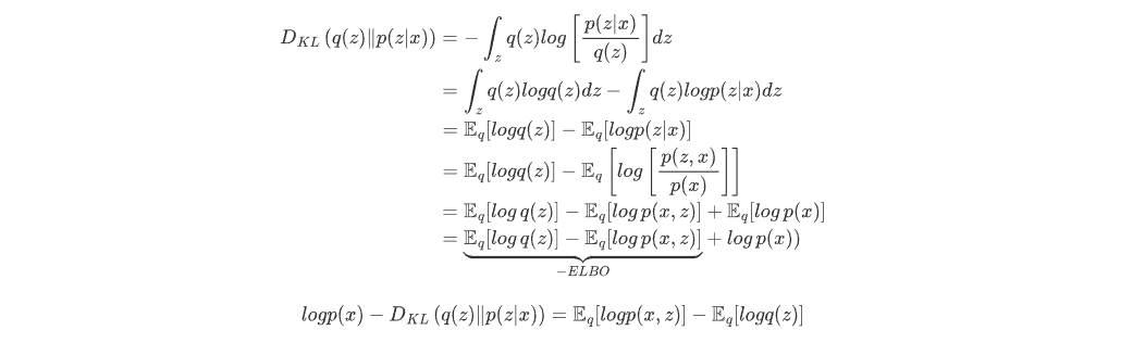
由于KL散度大于等于0，因此 $logp(x)>=\mathbb{E}_q[logp(x,z)]-\mathbb{E}_q[logq(z)]$ 。因此，当 $p(x)$ 分布难以计算时，常用最大化ELBO来近似最大化 $logp(x)$

三个假设：
- $p(z)=N(0,I)$
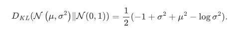
- $q(z|x)$ 服从各变量独立的标准正态分布，模型使用的假设是后验分布是正态分布。后验分布向标准正太分布靠近的过程中，防止了噪声为0，且保证了生成能力，达到了先验假设。
- $p(x|z)$ 服从各变量独立且方差为固定常数的高斯分布

高斯分布时，KL散度是有解析解的。隐变量为一维时有：

VAE的本质结构：重构的过程是希望没噪声的，而 KL loss 则希望有高斯噪声的，两者是对立的。所以，VAE 跟 GAN 一样，内部其实是包含了一个对抗的过程，只不过它们两者是混合起来，共同进化的。

前向过程：

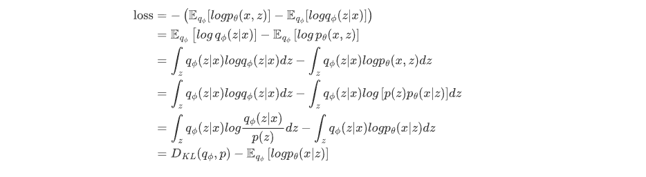
编码器用于拟合 $p(z|x)$ 的近似分布 $q(z|x)$ ，输出 $μ$ 和 $σ$ 。（变分后验分布的表达能力与计算代价的权衡一直是VAE领域的核心痛点）
从 $q(z|x)$ 中采样 $z$ ，解码器用于拟合似然分布 $p(x|z)$ ，输出 $μ$ ，方差为固定的超参。通过重参数化技巧得到 $z$ （因此重构过程受到噪声的影响，噪声的强度由方差决定，若方差为0，则模型退化为AE）
计算m次 $logp(x|z)$ 得到损失

VAE的缺点：

生成过程不可控
生成图片模糊，不同的 $x$ 可能采样得到相同的 $z$

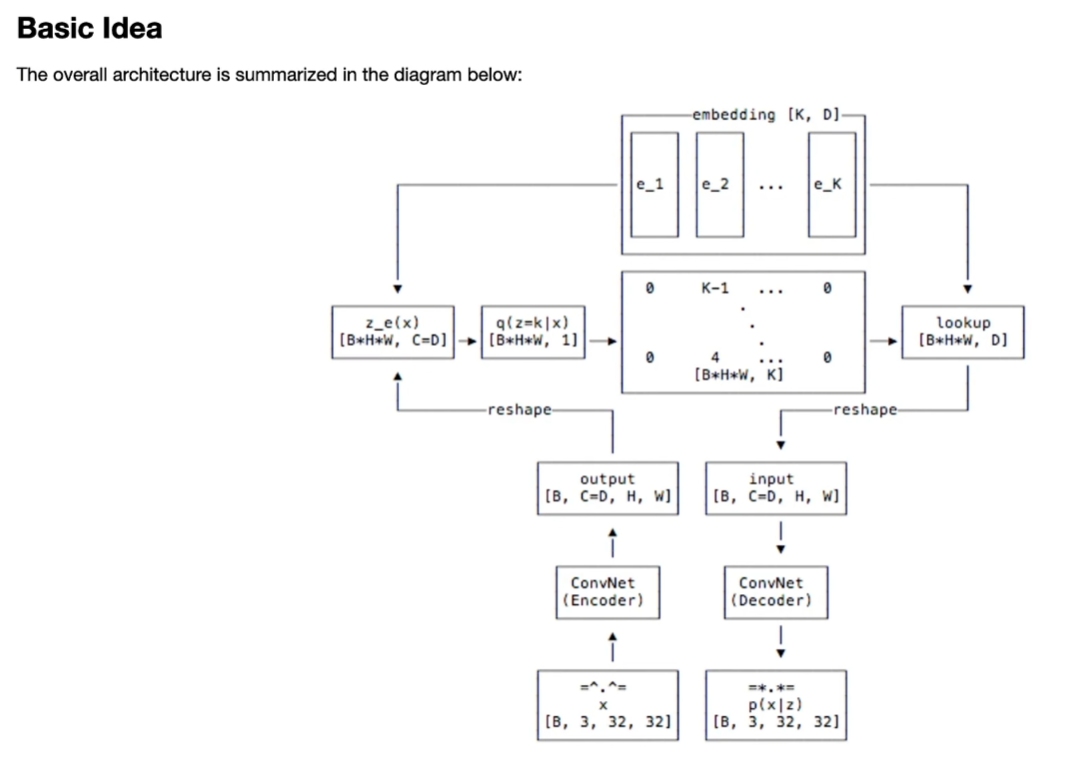
VQ-VAE

编码向量是离散的，先验分布不再固定（论文中先验分布是均匀分布与后验分布都是类别分布，两者KL散度为常数），可以避免后验坍塌的问题。

embedding space为[K, D]，编码器输出隐变量 $z_{e}(x)$ ，基于embedding space和 $z_{e}(x)$ 进行最近邻查找得到表征索引k，取出码本对应 $e_{k}$ 作为最终编码器的输出。 $\mathrm{k}=\mathrm{argmin}_j\|z_e(x)-e_j\|_2$

argmin导致不可导，将解码器输入部分梯度复制到编码器输出这部分，使得整个过程可导。

Diffusion model

背景

是否有一种生成模型，具有vae、gan、flow等模型的优点，只需要训练生成器，训练目标函数简单，不需要训练判别器或后验分布等，并且模型表达能力不受限。vae从数据分布->标准高斯分布->数据分布，diffusion从数据分布->标准高斯分布，生成器拟合逆过程即可。

训练过程

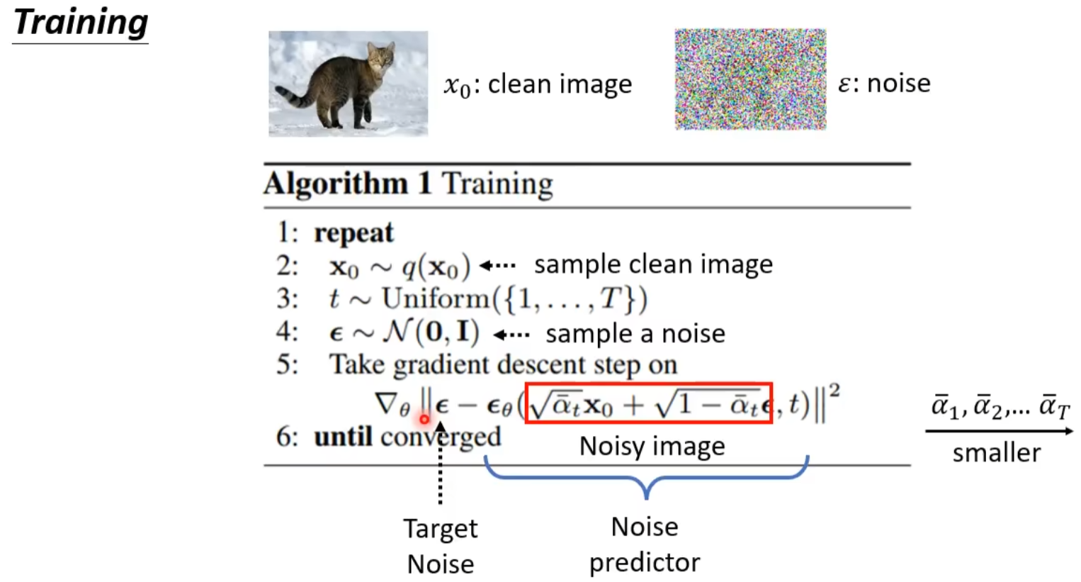
红框内的系数是为了控制不同时间步添加噪声的大小。

DDPM:

输入：噪声图像、时间步
输出：预测的噪声

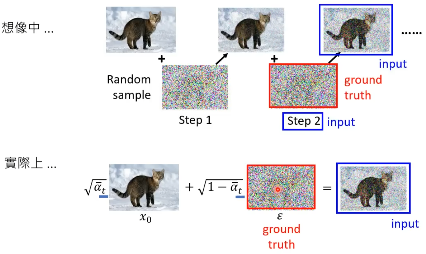
上图反映了 加噪过程 实际上并没有一步一步的加入噪声，而是一次就将噪声加进去， 去噪过程 也是一次就将预测噪声输出了。

推理过程

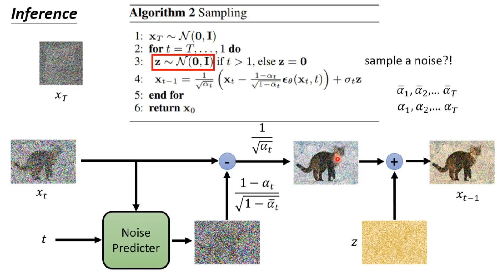
为什么DDPM中又加入了一次噪声才生成最终的去噪图片？

prediction裡加noise的概念在score-based generative model相關的paper中有提到，比較像是預測結果不應該收斂在一個特定的位置(a point in density region)，而是要在一個分布範圍(density region)。換句話說，如果每次update是得到一個向量(score function)朝向一個點，那noise就是讓這個向量(noisy score)轉換成朝向一個可能的範圍。讓結果從預測”一個固定方向”，轉成是要預測”一個固定範圍”，這只要sigma 足夠小，預測目標結果的分布範圍就會成立。

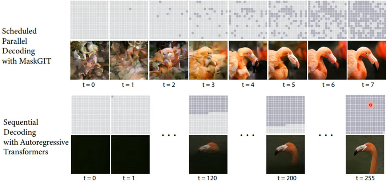
扩散模型可能不是那么重要，重点是怎么将一次生成加入自回归生成中。

DDPM核心代码

# 损失计算（https://github.com/abarankab/DDPM/blob/main/ddpm/diffusion.py）
def get_losses(self, x, t, y):
    noise = torch.randn_like(x)

    perturbed_x = self.perturb_x(x, t, noise)
    estimated_noise = self.model(perturbed_x, t, y)

    if self.loss_type == "l1":
        loss = F.l1_loss(estimated_noise, noise)
    elif self.loss_type == "l2":
        loss = F.mse_loss(estimated_noise, noise)

    return loss

def forward(self, x, y=None):
    b, c, h, w = x.shape
    device = x.device

    if h != self.img_size[0]:
        raise ValueError("image height does not match diffusion parameters")
    if w != self.img_size[0]:
        raise ValueError("image width does not match diffusion parameters")

    t = torch.randint(0, self.num_timesteps, (b,), device=device)
    return self.get_losses(x, t, y)

# 推理过程
@torch.no_grad()
def remove_noise(self, x, t, y, use_ema=True):
    if use_ema:
        return (
            (x - extract(self.remove_noise_coeff, t, x.shape) * self.ema_model(x, t, y)) *
            extract(self.reciprocal_sqrt_alphas, t, x.shape)
        )
    else:
        return (
            (x - extract(self.remove_noise_coeff, t, x.shape) * self.model(x, t, y)) *
            extract(self.reciprocal_sqrt_alphas, t, x.shape)
        )

@torch.no_grad()
def sample(self, batch_size, device, y=None, use_ema=True):
    if y is not None and batch_size != len(y):
        raise ValueError("sample batch size different from length of given y")

    x = torch.randn(batch_size, self.img_channels, *self.img_size, device=device)

    for t in range(self.num_timesteps - 1, -1, -1):
        t_batch = torch.tensor([t], device=device).repeat(batch_size)
        # 均值计算
        x = self.remove_noise(x, t_batch, y, use_ema)
		
        if t > 0:
            x += extract(self.sigma, t_batch, x.shape) * torch.randn_like(x)

    return x.cpu().detach()

# UNet中t是如何嵌入网络的
x = self.init_conv(x)

skips = [x]

for layer in self.downs:
    x = layer(x, time_emb, y)
    skips.append(x)

for layer in self.mid:
    x = layer(x, time_emb, y)

for layer in self.ups:
    if isinstance(layer, ResidualBlock):
        x = torch.cat([x, skips.pop()], dim=1)
    x = layer(x, time_emb, y)

x = self.activation(self.out_norm(x))
x = self.out_conv(x)

# 在残差块的前传中融入time_emb，类似加位置编码的过程
def forward(self, x, time_emb=None, y=None):
    out = self.activation(self.norm_1(x))
    out = self.conv_1(out)

    if self.time_bias is not None:
        if time_emb is None:
            raise ValueError("time conditioning was specified but time_emb is not passed")
        out += self.time_bias(self.activation(time_emb))[:, :, None, None]

    if self.class_bias is not None:
        if y is None:
            raise ValueError("class conditioning was specified but y is not passed")

        out += self.class_bias(y)[:, :, None, None]

    out = self.activation(self.norm_2(out))
    out = self.conv_2(out) + self.residual_connection(x)
    out = self.attention(out)

    return out

##引入条件的几种方式

输入端 Concatenation ，将其作为UNet输入中的额外通道进行输入。当条件特征与图像特征形状相同时，例如分割蒙版、深度图或图像的模糊版本（在恢复/超分辨率模型的情况下）时，通常会使用这种方法。它也适用于其他类型的条件。例如，类标签被映射到嵌入向量，然后扩展到与输入图像相同的宽度和高度，以便将其作为额外通道输入。

class ClassConditionedUnet(nn.Module):
  def __init__(self, num_classes=10, class_emb_size=4):
    super().__init__()
    
    # The embedding layer will map the class label to a vector of size class_emb_size
    self.class_emb = nn.Embedding(num_classes, class_emb_size)

    # Self.model is an unconditional UNet with extra input channels to accept the conditioning information (the class embedding)
    self.model = UNet2DModel(
        sample_size=28,           # the target image resolution
        in_channels=1 + class_emb_size, # Additional input channels for class cond.
        out_channels=1,           # the number of output channels
        layers_per_block=2,       # how many ResNet layers to use per UNet block
        block_out_channels=(32, 64, 64), 
        down_block_types=( 
            "DownBlock2D",        # a regular ResNet downsampling block
            "AttnDownBlock2D",    # a ResNet downsampling block with spatial self-attention
            "AttnDownBlock2D",
        ), 
        up_block_types=(
            "AttnUpBlock2D", 
            "AttnUpBlock2D",      # a ResNet upsampling block with spatial self-attention
            "UpBlock2D",          # a regular ResNet upsampling block
          ),
    )

  # Our forward method now takes the class labels as an additional argument
  def forward(self, x, t, class_labels):
    # Shape of x:
    bs, ch, w, h = x.shape
    
    # class conditioning in right shape to add as additional input channels
    class_cond = self.class_emb(class_labels) # Map to embedding dimension
    class_cond = class_cond.view(bs, class_cond.shape[1], 1, 1).expand(bs, class_cond.shape[1], w, h)
    # x is shape (bs, 1, 28, 28) and class_cond is now (bs, 4, 28, 28)

    # Net input is now x and class cond concatenated together along dimension 1
    net_input = torch.cat((x, class_cond), 1) # (bs, 5, 28, 28)

    # Feed this to the UNet alongside the timestep and return the prediction
    return self.model(net_input, t).sample # (bs, 1, 28, 28)

创建嵌入后，将其投影到与 UNet 内部一层或多层输出通道数量相匹配的大小，然后将其添加到这些输出中。例如，每个 Resnet 块的输出都添加了一个投影的时间步条件嵌入以及Stable Diffusion 中图像条件的嵌入方式。
网络中融入 Cross atttention （LSD）。当条件以某些文本形式存在时，这是最有用的 - 该文本使用变换器模型映射到一系列嵌入，然后在UNet中使用交叉注意力层将此信息合并到去噪路径中。
ControlNet 额外训练一个组件，不微调 SD

生成模型的目标

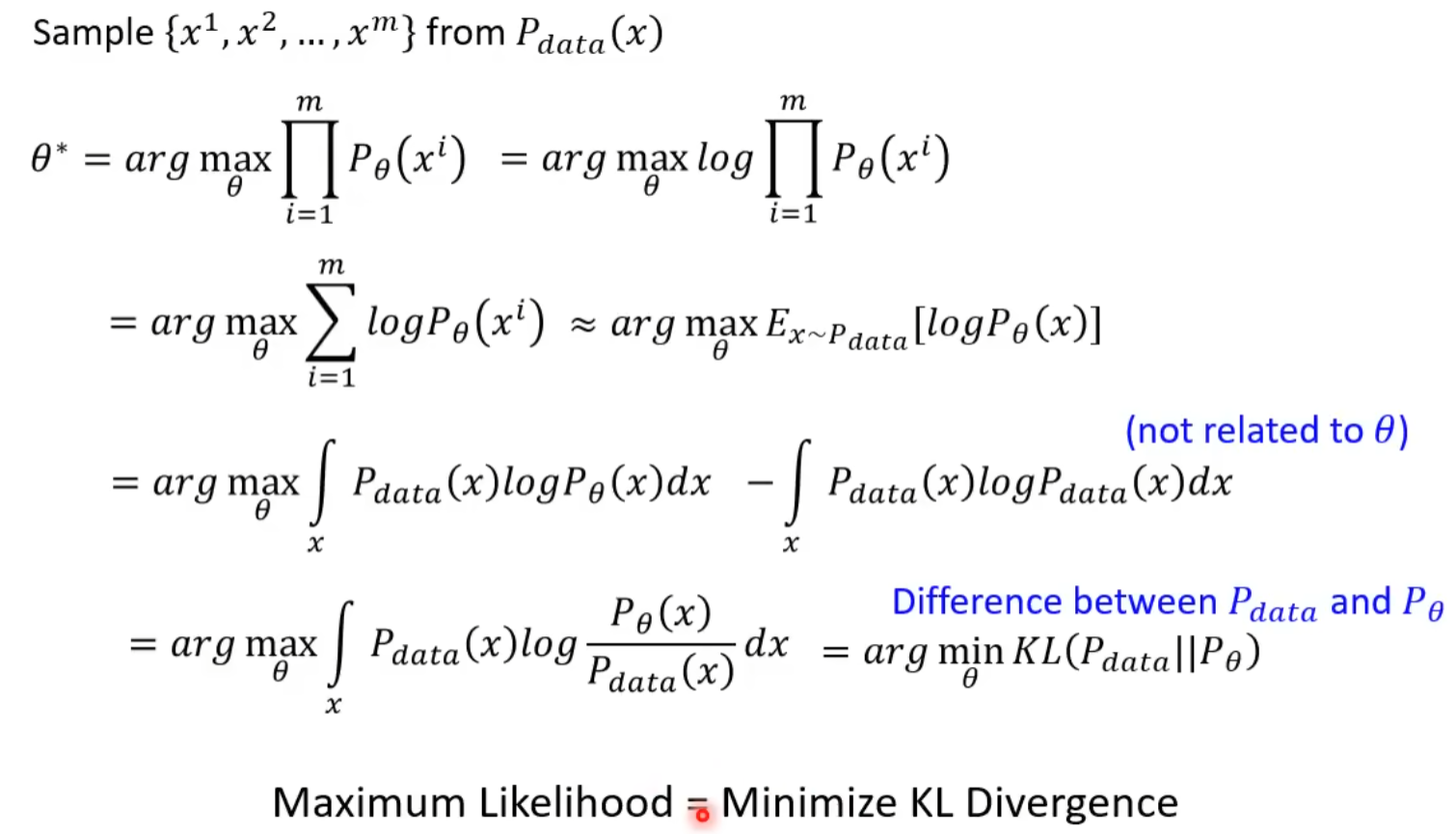
极大似然与KL散度的关联性

认知模态生成

Brain2img——方法总结

1. MindDiffuser

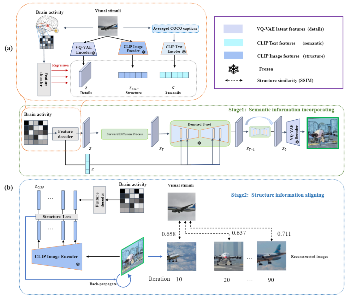
step1：训练三个全连接层直接将脑信号映射到不同的嵌入空间，然后使用训练得到的模型，输入 Brain activity 并使用得到的 z 、c 向量重构原图。（ 直接映射已经可以生成语义一致的图片 ，并没有设计复杂的对齐损失）

step2: 提取CLIP图像编码器的浅层线性层特征，如图2 (b)所示。然后，使用 fMRI 解码每一层对应的 CLIP 视觉特征，并计算两者之间的 L2 距离对齐结构信息。

Note： 仅仅使用了 mse loss ，对齐的约束只要有就可以，没有设计特定的对齐损失就取得了很好的效果。

定量指标：

CLIP相似度: 重建图像和原图在CLIP图像分支输出向量的余弦相似度，衡量二者的语义相似度
PCC: 重建图像和原图的皮尔逊相关系数，衡量二者的结构相似度
SSIM: 衡量二者的结构相似度
FID: 计算重建图像和原图分布的相似性，从整体上衡量重建图像的真实程度与多样性

Seeing through the Brain

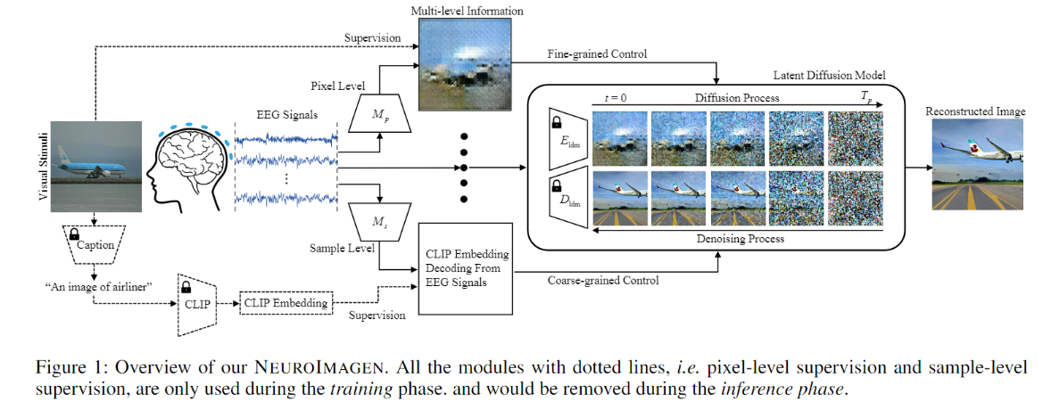
Pixel-level Semantics Extraction：扩散模型的输入是由生成器生成的粗粒度图像，而不是某个隐向量，需要单独训练一个生成器（额外的损失设计），增加了训练的负担。脑电与图片的对齐使用了对比损失
Sample-level Semantics Extraction：同样将对齐后的语义作为条件融合去噪过程，保证语义一致

Note： 脑信号的监督信号是预训练获得的 隐向量 还是 原始刺激

DreamDiffusion

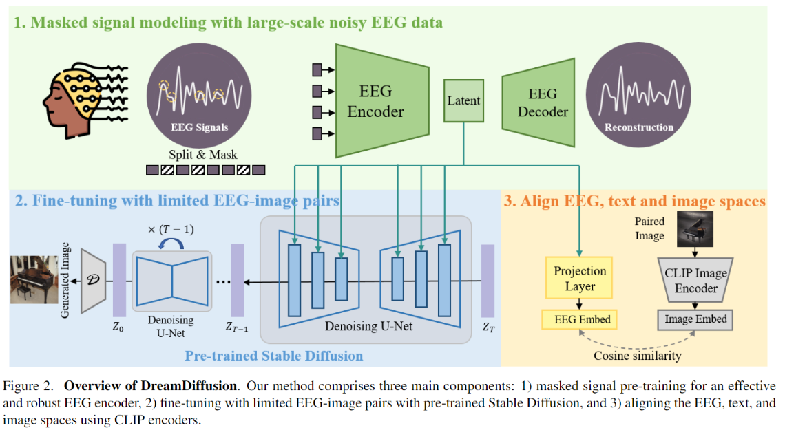
step1：利用了较大规模上预训练的EEG模型
step2：同时优化EEG编码器和UNet的cross-attention部分
step3：利用余弦相似度对齐EEG与图文，训练过程中会优化EEG编码器，使得对齐后的EEG_latent便于微调SD模型

Note：此处的对齐方式使用了余弦相似度，以上几篇基于扩散模型的方法中对齐损失都比较简单，没有设计和复杂的损失